


This essay is intended to offer a practical metric for evaluating changing limits and attachment points in a portfolio of excess policies.
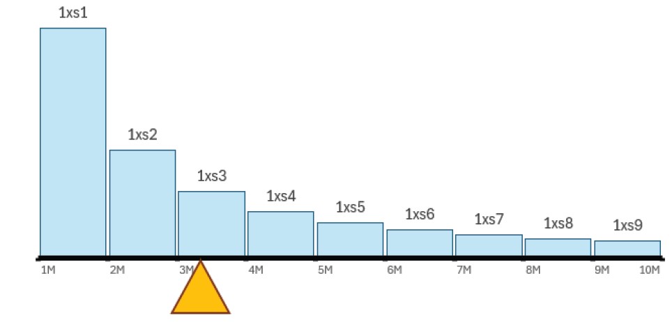
The problem arose in reviewing development patterns for a portfolio of excess policies that appeared to show changes from one accident year to the next. The team looked at average attachment points and policy limits by year but encountered difficulty in that analysis: Some layers had been split into smaller layers in recent periods. For example, what was previously a 9,000,000 excess of 1,000,000 policy is now three separate policies for 1,000,000 xs 1,000,000: 3,000,000 xs 2,000,000, and 5,000,000 xs 5,000,000. The quota share also varied across the three policies.
What is the correct way to estimate the average attachment point (or limit) for the new set of policies?
One suggestion that can help is to introduce a new metric: excess layer center of gravity (CoG).
The idea is to find a weighted average midpoint of the collection of policies. We can think of breaking the tower of layers more finely than even the three layers identified above; perhaps with a series of 1,000,000 limits in a tower. If we allocate premium to each of these smaller layers, we can then average the midpoint of each small layer by the allocated premium to get an overall CoG for the tower.
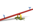
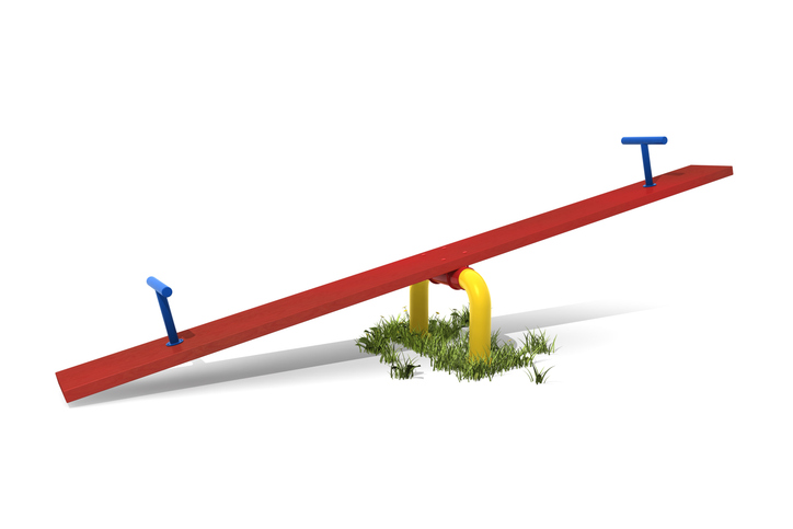
The idea of the CoG is derived from Archimedes’ “law of the lever,” but it may be more familiar from the playground experience of children on a seesaw.
If we consider the premium for contracts broken down into individual layers, then the CoG is the point where all the premium weights would be in balance. As more contracts are added to the portfolio, this CoG will shift with the weight of the new premium and the position of the layers. (See Figure 1.) This is the same as when more children climb onto the seesaw and try to keep it balanced.
Figure 1.
Mathematically, the CoG is defined as the following:
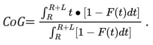
In this formula, the attachment point, or retention “R,” is the lower end of the layer, and the Limit “L” is the amount of coverage in excess of this retention that is provided by the policy. The limit should be expressed as 100% share, even if the policy is syndicated or coinsured by the policyholder.
The formula also ensures that the CoG is between the retention (R) and the upper limit (R+L), which is sometimes called the “plafond.” In fact, it will always be in the lower half of the layer as follows:
R < CoG ≤ R+L/2 .
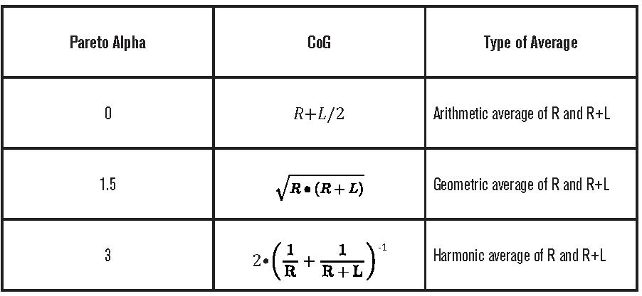
While the CoG formula is tractable for many severity distributions, the single-parameter Pareto gives some useful benchmarks to use as a shortcut.
A useful special case is the Pareto with shape parameter alpha equal to 1.500. The CoG is equal to the geometric average of the retention and the upper limit (plafond). For example, a layer of 5,000,000 excess of 5,000,000 would use the square root of the product of 5,000,000 and 10,000,000: resulting in a CoG of 7,071,068. As the shape parameter moves towards zero, the CoG moves towards the midpoint of the layer.
Three common types of averages are each special cases of the single parameter Pareto (see Table 1).
Table 1.
If premium is allocated to layers using the same Pareto as for the CoG statistic, the portfolio CoG is not distorted by how the layers are split or combined. This is shown in Table 2. The layers are in proportion to expected loss from a Pareto with alpha equal to 1.500. The overall CoG is then a premium-weighted average of the individual CoG statistics.
Table 2.
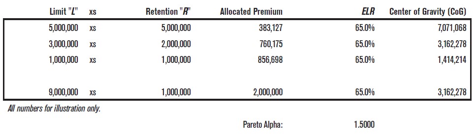
In practice, we use the actual premium by layer, which reflects the share of each layer in the portfolio. But the limit in the calculation should always be at 100% share.
As an example of changing quota share, we might change the 5,000,000 xs 5,000,000 layer to instead take a 50% share of 10,000,000 xs 5,000,000. The retention and “net” limit are not changed, but the CoG does move. The CoG shifts from 7,071,068 (geometric average of 5,000,000 and 10,000,000) to a CoG of 8,660,254 (geometric average of 5,000,000 and 15,000,000). The higher CoG may imply a slower development pattern.
The Pareto assumption is also not necessary. If a more detailed library of size-of-loss distributions is available, then the CoG statistic can be further refined. The geometric average based on Pareto alpha = 1.500 is merely a convenient starting point.
The information needed by excess policy is:
-
- Amount of premium
- Retention (or “attachment point”)
- Policy limit at 100%
The CoG statistic gives us another summary statistic for our portfolio that can be tracked over time. We would expect that if the CoG is increasing at approximately the rate of inflation then the development pattern should be stable. Otherwise, a change in CoG may help to explain a speed up or slowdown in the development. (The speed of development relative to CoG should be similar to the relationship to the Retention, as described by Pinto & Gogol in their 1987 PCAS paper “An Analysis of Excess Loss Development.”)
The advantage is that it combines the effects of the retention, limit, and quota share into a single metric that can be averaged consistently across layers.
As a simple metric, it will not help as much with evaluating volatility. It also will not pick up development pattern changes due to other features such as annual aggregate deductibles (AADs) or loss ratio caps.
What other metrics do you use to track changes in the portfolio in reserving?
Dave Clark, FCAS, is a senior actuary with Munich Re.