
In experience rating calculations, the weight assigned to historical years is typically based on some volume measure. This treats each year as equally predictive of the prospective period.
In practice, actuaries recognize that older years may be subject to uncertainty in pricing parameters (e.g., trend and rate on-level indices) and changing risk profiles over time. The more recent periods are more representative of the prospective period than are older years as they recede into the past.
Several models have been suggested for assigning decreasing weights as the relevance of older years decreases (see references). This essay will describe a small recursive formula for setting these weights as a compromise between two extreme cases. It is a formula for how quickly we want to forget old experience.
The first case would be a pure auto-regressive model, AR(1), or “random walk.” In this case, each historical year would have a variance contribution proportional to its distance in time. A period only one year from our forecast period would have variance of 1∙s2AR1; the next year back would have variance of 2∙s2AR1; the year before that would have variance of 3∙s2AR1, and so forth.
In the autoregressive model, the covariance structure is shown below as matrix V. The vector of weights assigned to the historical years is equal to the row totals1 of the inverse of the covariance matrix. This results in all the weight assigned to the most recent year, and no weight given to any of the older years.
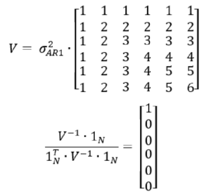
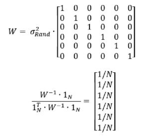
The other extreme is the case where all of the pricing parameters are known with certainty and the risk portfolio has been stable over time. This means that the covariance matrix follows an “independence” structure and implies equal weights assigned to each historical year.
The compromise between the two approaches is derived by combining the two covariance matrices, with the result being a smooth pattern giving more weight to recent years. Under our simplifying assumptions, the weights by year can be calculated easily with a recursive formula, without the need for any matrix operations (Excel users rejoice!).
The recursive formula can be put into an alternative form, with the choice of implementation being only a matter of convenience. The final weights by year just normalize the D_k sequence to sum to 100%.
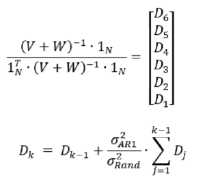
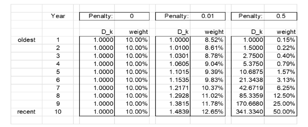
The recursive formula is set up with a “penalty” value s2AR1/s2Rand, where the numerator is the autoregressive variance from the pricing parameters and the denominator is the random variance of the losses. The penalty value can change from one analysis to another, depending upon the relative contributions of these two sources of variance. When this penalty is zero, we assign equal weights to all years (we never forget). As the penalty grows, the older years are more rapidly forgotten.2
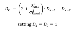
Table 1 shows some results for selected penalty amounts. It can be easily adjusted for other penalty amounts or number of years included.
Table 1.
This example is only a small special case; more sophisticated and realistic variance and covariance structures are possible. The interested reader is encouraged to explore the broader literature in the references.
References
- Fackler, Michael, “Experience rating of (re)insurance premiums under uncertainty about past inflation,” Ph.D. thesis, Uni Oldenburg (2017). https://oops.uni-oldenburg.de/3227/.
- Gluck, Spencer, “Balancing Development and Trend in Loss Reserve Analysis,” Proceedings of the Casualty Actuarial Society (1997).
- Korn, Uri, “An Extension to the Cape-Cod Method with Credibility Weighted Smoothing,” CAS E-Forum (2016).
- Mahler, Howard, “Credibility with Shifting Risk Parameters,” PCAS (1998).
- Riegel, Ulrich, “A Generalized Loss Ratio Method Dealing with Uncertain Volume Measures,“ ASTIN Bulletin (2018).
Dave Clark, FCAS, is a senior actuary with Munich Re.
1 The 1N term in these equations represents a vector of all 1s, of length equal to the number of columns in the matrix. This is a way of taking row totals in matrix operations.
2 While not directly useful for insurance pricing, it is interesting to note that when the penalty is 1.00, then the weights follow a pattern related to the “golden ratio” (phi). Fackler describes the more general case as part of Fibonacci Algebra (section 4.3.2).


