


In my “Explorations” that appeared in the July/August 2015 edition of the Actuarial Review, I reported on my progress in working with the bivariate stochastic loss reserve model proposed by Zhang and Dukic.1 Here is a summary of what they did.
They took a stochastic Bayesian MCMC version of a well-established loss reserve model. Using that model to describe the marginal distribution of outcomes for each of two lines of insurance, they fit a bivariate distribution that allowed for dependencies between the two distributions as described by a copula. Using Bayesian MCMC software, they then generated a predictive distribution for the joint distribution of the two lines. This predictive distribution consisted of the parameters of the model for each line, and the parameters of the copula. A feature of the Zhang/Dukic approach was that there was no guarantee that the parameters of the bivariate model would agree with the parameters of a univariate model fit to a single line’s data. As it turned out, this was a problem for my changing settlement rate (CSR) model.2
After some thought, I was able to come up with a way to generate a sample from the predictive distribution for a bivariate stochastic loss reserve model that preserved the univariate marginal distributions.3 Having done that, I then turned to a more interesting question: How does this bivariate model that allows for dependencies compare to an alternative bivariate model that assumes independence between the lines of business?
To answer that question I had to learn more about model selection statistics for predictive distributions. My “Explorations” column in the March/April 2016 issue describes some of what I learned — namely that something called the WAIC statistic allows one to indicate model preference while taking the number of model parameters into account.
I then fit bivariate CSR models to the 102 pairs of within insurer lines of business that I analyzed in my monograph, with the surprising result that the WAIC statistics favored the independent bivariate model for all 102 pairs of lines!
In discussing this result with my actuarial colleagues, I found that others were also surprised, or even skeptical of my results. The skeptics pointed to common drivers of dependency such as inflation or the underwriting cycle.
One feature of the CSR model is that it allows the expected loss ratio to vary significantly by accident year. This is in contrast to some favorite models of many actuaries such as the Bornhuetter-Ferguson or Cape Cod models that force the expected loss ratio to be constant across accident years.
With this contrast between the CSR and the current actuarial favorites, I built a model that assumes that the expected loss ratio is constant across accident years. I called this model the “Stochastic Cape Cod” (SCC) model. Proceeding as above, I found several instances where the bivariate SCC model that allowed for dependencies was preferred to the bivariate SCC model that assumed independence.
Insurer #5185 in the CAS Loss Reserve Database provides a good example to examine in detail. If we select a single parameter set from the posterior distribution we can construct a set of 55 standardized residuals

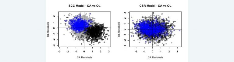
where Cwd is the cumulative paid loss for accident year w and development year d in the 10 x 10 data triangle. μwd and σd are the mean and standard deviation calculated from the selected parameter set from the posterior distribution of the model. Repeat this for a sample of 100 parameter sets selected at random from the SCC and CSR models. The exhibit below shows plots of the standardized residuals of the sampled parameter sets (5,500 points in all) for both models for the Commercial Auto (CA) and the Other Liability (OL) lines of insurance.
- The first row shows plots of the standardized residuals against the accident year for CA.
- The second row shows plots of the standardized residuals against the accident year for OL.
- The third row plots the standardized residuals for CA against the corresponding standardized residuals for OL. The plot for each point consists of a solid gray circle. A black border surrounds the points for accident year one. A blue border surrounds the points for accident year three.4 The posterior mean of the coefficients of correlation between the log(Cwd)s are -0.40 for the SCC model and -0.02 for the CSR model.

In a well-fitting model, we should expect to see the residuals normally distributed around zero for the accident year plots. This is the case for the CSR model, but is not the case for the SCC model. In this case the bulk of deviations from zero have the opposite signs for the same accident year in the different lines of insurance. This leads to a significant negative correlation for the SCC model.
In examining other pairs of triangles with different insurers, I often see the paired residual plots by accident year occupy distinct regions in the plane. If the regions are mainly in the northwest and southeast quadrants, we will see a negative correlation as we did for insurer #5185. It is also possible for the accident year regions to be mainly in the northeast and southwest quadrants resulting in a positive correlation. Another possibility is for the accident year regions to be in all four quadrants resulting in a near zero correlation.
Since the CSR model allows the expected loss ratio to vary by accident year, there are no distinct accident year regions.
The takeaways that I get from this exercise is that first we can fit a bivariate stochastic loss reserve model that captures any dependencies between two lines of insurance. Second, if we see evidence of some dependency, we should look for a better model.
These results will have a significant impact on the liability risk margin formula put forth in Solvency II, which does not recognize the effect of diversification by line of insurance. I plan to discuss this in a later column.
1 Zhang, Yanwei and Vanja Dukic. 2013. “Predicting Mulitvariate Insurance Loss Payments Under the Bayesian Copula Framework.” The Journal of Risk and Insurance, Vol. 80, No. 4, 891-919.
2 The CSR model is described in my monograph that is available on the CAS website at http://www.casact.org/pubs/monographs/index.cfm?fa=meyers-monograph01
3 A preliminary version of my paper describing how to do this appears in the CAS E-Forum, Winter 2016. I submitted a later version of the paper to a peer-reviewed journal.
4 I chose accident years one and three because they illustrate the point most dramatically.