


The title of this essay is taken from a comment made by David Spiegelhalter on the original thought experiment of Thomas Bayes, introducing the ideas behind what became known as Bayes’ Theorem.
The thought experiment is found in Bayes’ “An Essay towards solving a Problem in the Doctrine of Chances,” edited and published (1763) by his friend Richard Price. The goal of Bayes’ essay was to quantify “inverse probabilities.” That is, how to estimate the probability of some state of the world having observed some experimental data.
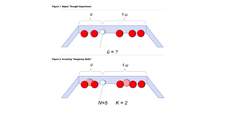
To address this problem, Bayes set up a thought experiment for randomly rolling balls on a long table. In the initial setup, a white ball is rolled on the table in such a way that it could randomly land anywhere, and its position is unknown to the experimenter. In the second step, a number of red balls are rolled on the table also randomly and with their exact locations not known to the experimenter. The only information known is how many red balls, P, are to the left of the white ball, and how many, Q, are to the right of the white ball. (See Figure 1.)
Knowing only the numbers P = 2 and Q = 3, can we make a statement about the probability that the white ball is between any two points X1 and X2? For example, if we assume that each red ball has an equal probability of rolling to any point from 0 to 1, what is the probability that u is between 0.40 and 0.50? Bayes gave an answer to this by estimating a series expansion for what we would now recognize as a beta distribution.
Prob(X1 ≤ u ≤ X2|P,Q) =
(∫X1X2 uP∙(1-u)Q du) ⁄ (∫01 uP∙(1-u)Q du)
If we want a point estimate of the parameter u, the expected value is found as:
E(u|P,Q) = ((P+1)/(P+Q+2))
We would estimate the position of the white ball as u = 3/7 based on this formula. This differs from the maximum likelihood estimate of P/(P+Q) = 2/5. The expected value has an extra “1” in the numerator and a “2” in the denominator.
Unlike the maximum likelihood estimate, the conditional expected value never reaches either 0 or 1. Even if all of the red balls are to the right of the white ball, we do not estimate u = 0.
The additional 1 in the numerator and the 2 in the denominator act as ballast and are based on the “prior knowledge” that the white ball was equally likely to have landed anywhere on the table. Spiegelhalter (2021) notes the connection to data augmentation because the prior knowledge can be viewed as “imaginary balls,” one on either side of the line separating left and right.
“In fact, since Bayes’ formula adds one to the number of red balls to the left of the line [position of white ball] and two to the total number of red balls, we might think of it as being equivalent to having already thrown two ’imaginary’ red balls, and one having landed at each side of the dashed line.” (Page 325.)
This is a remarkable idea: Our prior knowledge (that the white ball could be anywhere on the table) can be introduced either as an explicit prior beta distribution, or in the form of data augmentation (adding imaginary balls).
The expression for the posterior expected value can also be written in the familiar credibility form:
E(u|P,Q) =
(P/(P+Q))∙(N/(N+K))+(1/2)∙(K/(N+K))
N = P+Q, K = 2
In the credibility form, N is the number of actual balls observed, and K is the number of imaginary balls representing the prior knowledge.
For actuaries, this example is instructive because it provides an alternative interpretation to the familiar credibility constant K. In the usual Bühlmann interpretation, K is equal to the ratio of the expected process variance (EPV) to the variance of hypothetical means (VHM). But K can also be viewed as the amount of pseudo-data (imaginary balls).
Including our prior knowledge in the form of pseudodata is a simple but powerful way to perform a blending of observed loss experience with prior knowledge. The method is not limited to Bayes’ billiard balls but can be expanded to other models such as generalized linear models (GLM) as described in Huang, et al., where noisy data in predictive models can be stabilized by introducing a small amount of imaginary data.
They note:
“The practice of using synthetic data (or pseudo data) to define prior distributions has a long history in Bayesian statistics. It is well known that conjugate priors for exponential families can be viewed as the likelihood of pseudo observations.”
The idea of incorporating prior knowledge in the form of pseudo data to augment observed loss data may be a fruitful area of future research for actuarial models.
References
Huang, Dongming, Nathan Stein, Donald B. Rubin, and S.C. Kou. “Catalytic prior distributions with application to generalized linear model.” Proceedings of the National Academy of Sciences (PNAS) 2020 Vol. 117 (22); 12004-12010.
https://www.pnas.org/doi/10.1073/pnas.1920913117.
Spiegelhalter, David. The Art of Statistics: How to Learn from Data, Basic Books, 2021.