


aggregate is an open-source Python package available for free online that I’ve been developing since 2017. The following example shows how you would use it in practice — and check out a video tutorial in the link section at the end of this article.
You are the risk manager for ABC Trucking, Inc. ABC has a captive providing commercial auto liability insurance for its fleet with a $10 million occurrence limit. You manage the captive’s net exposure using per occurrence reinsurance and an aggregate stop loss. Your goal is to buy reinsurance to keep the 99th percentile of your net loss around $3.5 million. Previously, you relied on a simple Excel spreadsheet and some broker rules of thumb to guide your purchases. This year, you will use new software called aggregate to model your gross and net risk.
The documentation (see links below) explains that you need to start by installing the software. You fire up your favorite Python interface (e.g., Jupyter Lab or RStudio) and enter:
!pip install aggregate
First, you need to specify the gross distribution of losses for your portfolio. This is done using the Dec Language (DecL), a human-readable way to go from a declarations (dec) page to a frequency-severity probability distribution. The DecL for your account has six clauses:
Agg ABC.Gross
exposure
limit
severity
occurrence reinsurance
frequency
aggregate reinsurance
agg is a keyword, like select in SQL, instructing DecL to create an aggregate distribution. ABC.Gross is a label. The remaining clauses contain your specific details.
exposure describes the volume of risk. Your actuary’s expected loss cost is $5 million, and they estimate severity of $38,236, giving an expected claim count of 130.8. The exposure clause is 130.8 claims, which can be specified using a Python f-string as f'{5e6 / 38236} claims'. The f-string substitutes the values into the string.
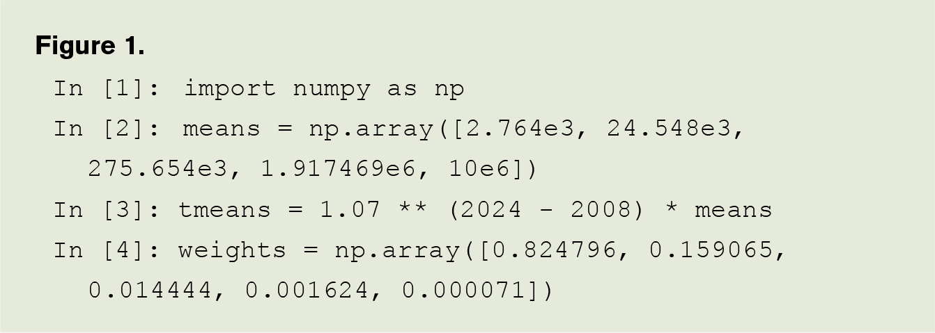
The severity clause specifies the unlimited size of loss distribution. A lognormal distribution with mean 50 and CV 4.5 is simply sev lognorm 50 cv 4.5, and you can probably guess the form for a gamma or other commonly used severity distributions. All scipy.stats distributions are available. Your actuary recommends using a mixed exponential severity, heroically trended from an old CAS presentation with means and weights as follows as shown in Figure 1.
The DecL is entered as f'sev {tmean} * expon 1 wts {weights}', where sev is a DecL keyword and expon 1 specifies a standard exponential distribution with mean 1.
There is no reinsurance for the gross portfolio — we’ll come to that later. The frequency clause specifies the claim count distribution. Your actuary recommends a gamma-mixed Poisson distribution with a mixing CV of 20%, producing a negative binomial. The DecL is mixed gamma 0.2.
The next step is to use aggregate to build the compound probability distribution from its DecL specification. Returning to Python, you import build and qd from the library and run a short program. The build object provides easy access to all functionality, and qd is a quick-display function providing formatted printing. You can enter the gross portfolio DecL as show in Figure 2, using line breaks for clarity, since Python automatically concatenates strings between parentheses.
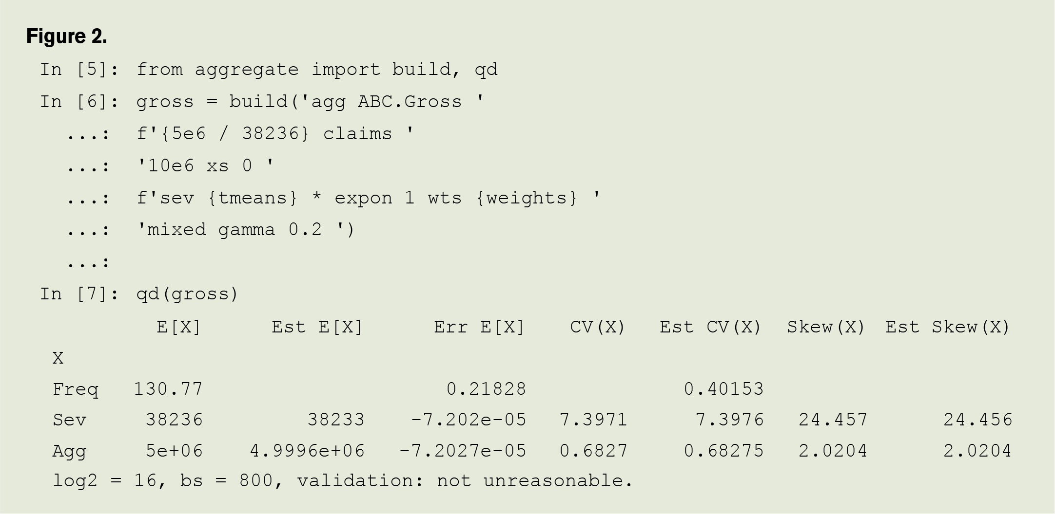
What has this done? aggregate has created a discrete approximation to the severity distribution using 216=65536 buckets of size 800. Then, it uses a Fast Fourier Transform (FFT) algorithm to compute the convolutions and aggregate distribution. Separately, it computes the expected mean, CV, and skewness for limited severity and the aggregate distribution analytically and compares them with the FFT routine. These statistics are reported by qd(gross). The mean has a relative error of 7.2e-05, and the CVs and skewnesses agree to four significant digits. The last line reports that all validation tests pass: the approximation is “not unreasonable.” (Validation is like a null hypothesis; not failing is the best result.)
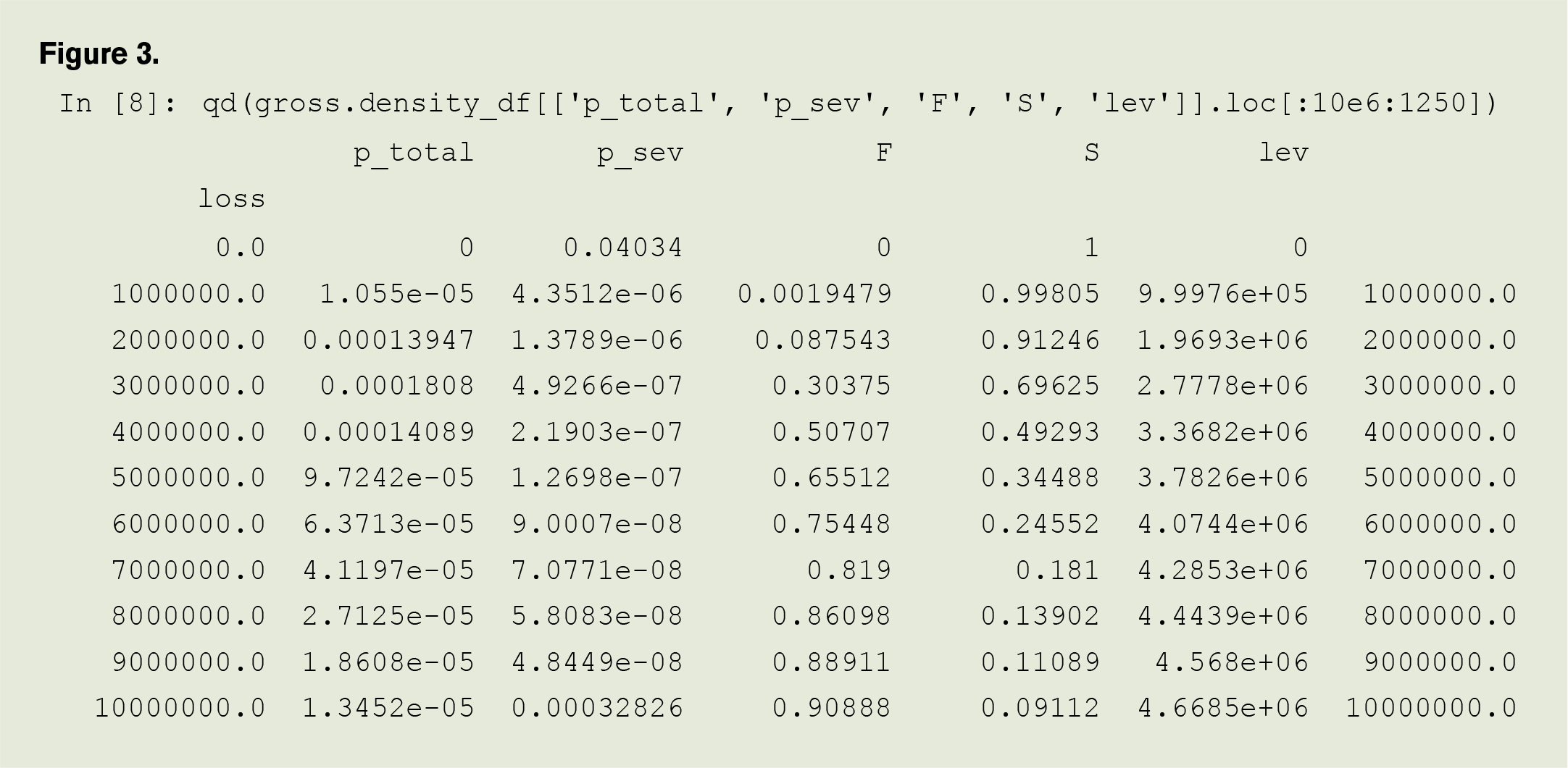
The discretized severity and aggregate distributions are stored in a Pandas dataframe that can be accessed and manipulated using Python code, such as that shown in Figure 3. The function qd here just provides sensible number formats. p_total and p_sev are the aggregate and severity probabilities, F and S are the aggregate cdf and survival function.
Now, you want to apply occurrence reinsurance. You usually buy a tower starting at $250,000 with a co-participation, building up to the $10 million occurrence limit. The DecL clause occurrence net of 50% so 250e3 xs 250e3 applies a 50% share of (so) the $250,000 xs $250,000 layer, with unlimited reinstatements. Layers can be chained together. Your full program is as shown in Figure 4.
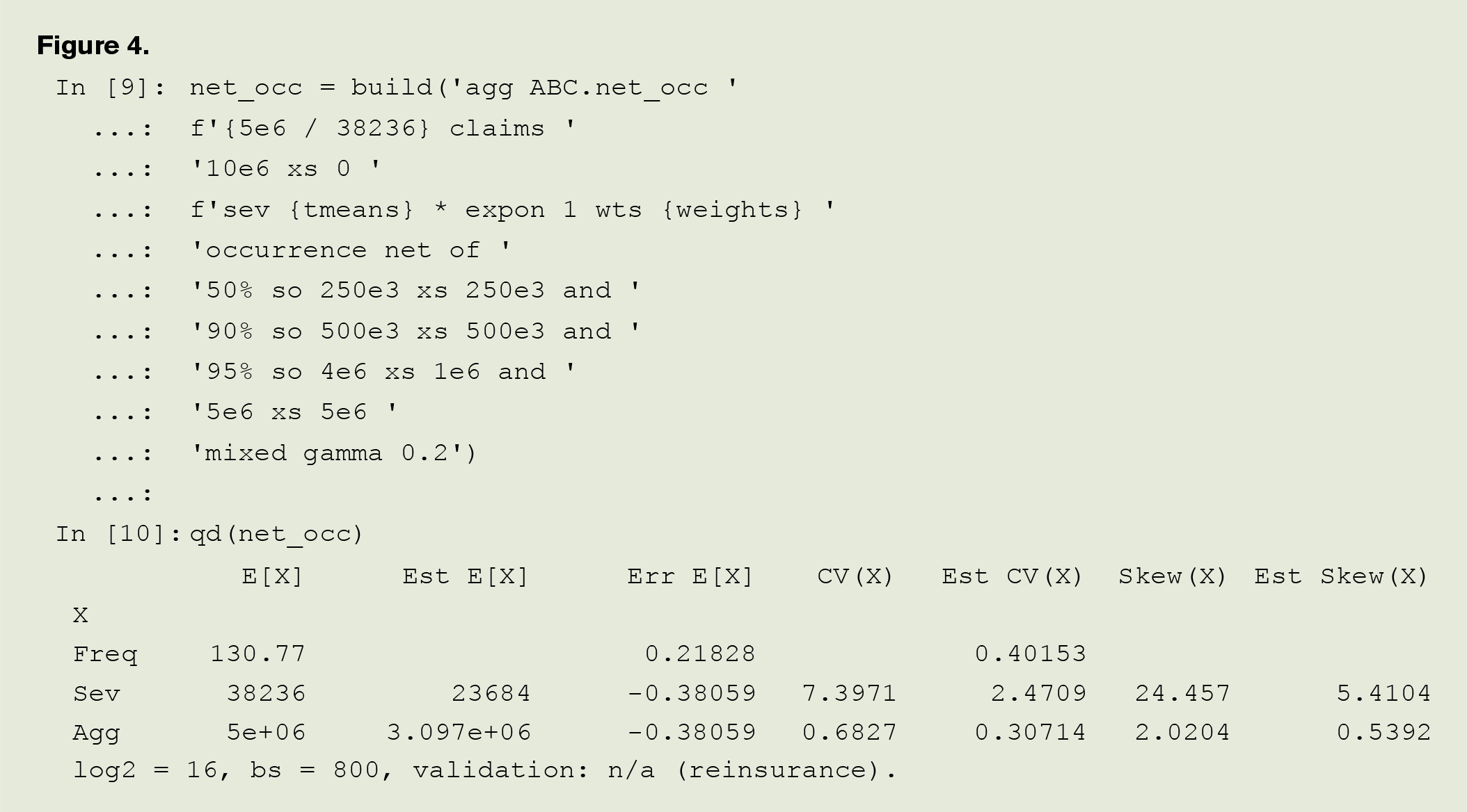
The reported Est[imated] statistics now refer to the net result. This has lowered the expected loss from $5 million to $3.1 million and reduced the portfolio CV from 68% to 31%. An objective of aggregate is to make working with frequency-severity distributions as easy as working with the lognormal, with standard probability functions built in. The cumulative distribution function (cdf) and quantile function (inverse of cdf, aka VaR function) are accessed as
In [11]: gross.cdf(3.5e6), net_occ.cdf(3.5e6), gross.q(0.99), net_occ.q(0.99)
Out[11]: (0.41186030905343524, 0.6902259054503352, 16984000.0, 5672000.0)
The occurrence reinsurance has reduced the 99th percentile loss from $17 million to $5.7 million. Your target 99% loss is only $3.5 million. To get there, you model an aggregate stop loss to attach at $3.5 million and cover up to $5.7 million as seen in Figure 5.
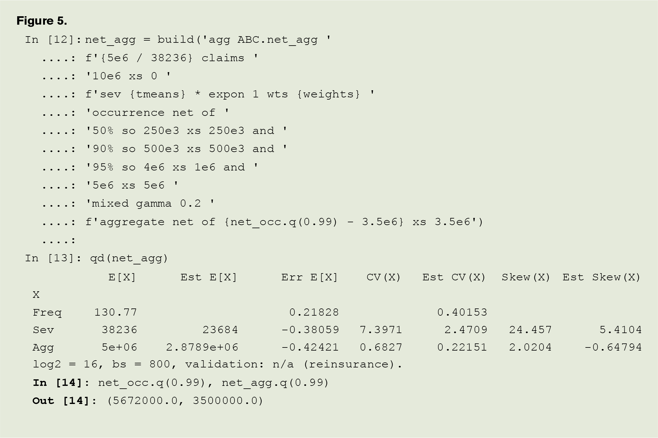
Net losses now have a mean of $2.9 million and CV of 22%. The last line confirms the 99th percentile achieves the $3.5 million target.
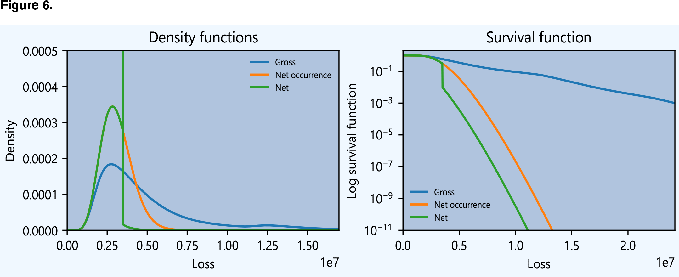
From here, a few lines of standard Python code can produce graphics and visualizations (see Figure 6).
I hope this short example gives you a feel for the power of aggregate. I used it to create all the case study exhibits and figures in my book with John Major, Pricing Insurance Risk (see Richard Goldfarb’s book review in AR, November-December 2022). If you install it, you can recreate those exhibits and create your own for different portfolios. You can read more about it in the documentation, and the source code is on Github. There is also a series of short videos on YouTube.
Links
- Documentation: https://aggregate.readthedocs.io/en/latest/
- Source code: https://github.com/mynl/aggregate
- Videos: playlist https://youtube.com/playlist?list=PLQQxycbewjqMDmw0hfZdB6Rzm60Qcq3Ao and a video on this specific example at https://youtu.be/nLMmhbFVHyw
- Scipy.stats distributions list: https://docs.scipy.org/doc/scipy/reference/stats.html
- The mixed exponential parameters: https://www.casact.org/sites/default/files/presentation/rpm_2011_handouts_ws1-zhu.pdf. The means and weights shown on slide 24 are trended from 2008 to 2024 at 7% per year.
- Actuarial Review: https://ar.casact.org/fairness-for-insureds-and-investors/
- Jupyter Lab workbook: https://colab.research.google.com/drive/1gKO4zJfhqR_difNyKHBdSbq0IK5gP1X9?usp=sharing
- Video walk-through: https://youtu.be/nLMmhbFVHyw
Stephen Mildenhall, FCAS, CERA, Ph.D., MAAA, ASA, CCRMP, CSPA, is retired with over 25 years of experience in the insurance industry and academia. He now spends far too much time programming in Python.