


In November, Late Last Year …
Kim Hypothetical, FCAS, is a pricing actuary in the Large Accounts department at Hypothetical Insurance (no relation). It is just before lunch. Kim wonders, “Is traditional actuarial work the best choice for me? Maybe I should be a predictive modeler.” Kim makes a note to investigate the new iCAS credential …
Hypothetical’s Chief Enabler of Opportunities walks over to Kim’s tiny open-plan solution conception pod. A rush project has just come in from their favorite broker at Gal Benmeadow. Lectral College, a large claims administration client of Gal’s and Hypothetical’s, is worried about its aggregation risk. Lectral has locations in every state and a substantial total exposure. The broker wants to structure an aggregate stop loss attaching “in the middle of the distribution.” Good news: The account has wonderful data, some of it stretching back to the Declaration of Independence — although it may not all be relevant today. The CEO asks Kim to work up some numbers to review before the end of the day.
Over lunch, Kim ponders the assignment. Straightforward. The claim history will be enough to build a frequency and severity model. The frequency of claims: Poisson. Trend and develop historical losses; use Kaplan-Meier to handle limited claims and fit an unlimited severity distribution. Then frequency-severity convolution applying the prospective limits profile. Throw in the Heckman-Meyers method to impress the CEO, Kim thinks. No need to change my dinner reservation, I will be done before six. The hardest part will be translating what the broker meant by “in the middle of the distribution.”
Back at the solution conception pod, Kim opens the submission and begins investigating the data. It is true there is an extensive claims history; Kim cannot recall having seen better data. A couple of clicks and Kim has a summary of historical claim frequency by state. It turns out Lectral has only one location per state, and almost all of its locations have had a claim at one point or another. There are so many years of data it is hard to know how much of the data to use. Kim settles on using losses since 1972.
Claim severity contains a surprise. Lectral’s losses are all full-limit losses. There is just a single partial loss in the history, in 2008, and that was a small loss. I can think of it as a stated amount policy, Kim thinks. That will simplify the analysis. The broker has even provided a prospective limit profile, which can be used in place of severity. Dinner’s a lock, Kim thinks.
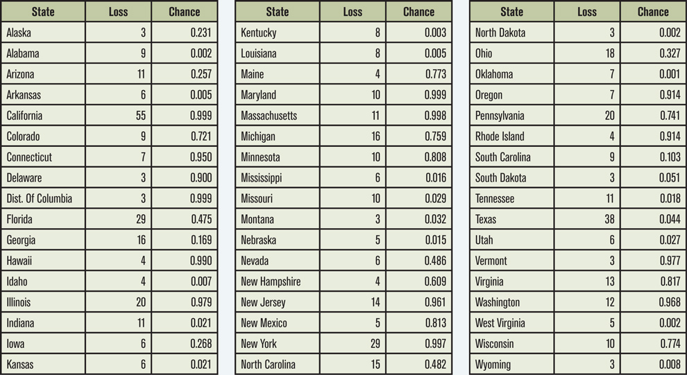
Kim summarizes the probability of loss ps and the stated-amount ls for each state s (Table 1). Aggregate losses L=∑slsBs where Bs is a Bernoulli random variable with parameter ps. Kim’s first thought is to simulate the distribution of L, but then Kim has a better thought: fast Fourier transforms.
With a few lines of Python, Kim writes a function agg taking inputs ps and ls and returning the full distribution of losses.
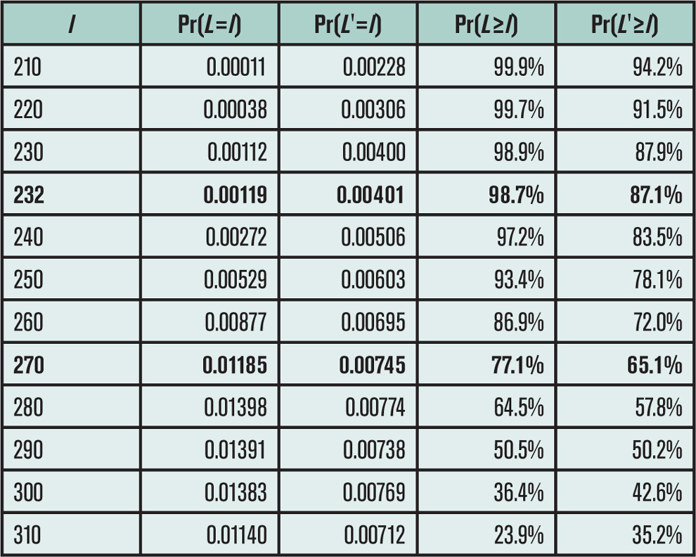
After less than an hour on the project, Kim has the full distribution of aggregate losses (Figure 1, Table 2) and is ready to price whatever structure the broker proposes. The mean loss is just above the midpoint. In fact, there is a 77.1 percent chance of a loss greater than 50 percent of the aggregate limit. Next step: Review with the CEO.
Hypothetical Insurance prides itself on its sophisticated pricing methods. It is particularly proud of its profit load algorithm, the PLA. The PLA was developed by a famous actuary many, many years ago. Central to the PLA is the idea of splitting account-level risk into process and parameter risk components and charging separately for each. Hypothetical believes all risk should be compensated and even applies a charge to process risk, unfashionable though that may be. The CEO likes to point out that Hypothetical was spared a New Zealand earthquake loss by the PLA-enforced pricing discipline. Rating agencies are impressed with its risk management. In line with modern financial thinking, Hypothetical also understands systemic parameter risk is more significant and so it is given a much larger weight in the PLA.
The CEO reviews Kim’s exhibits. “Full marks for working efficiently and nice use of the FFT! I’m glad you saw so quickly you do not need to worry about severity — I forgot to mention that to you. But what about the risk loading?”
Kim is annoyed. How could I have forgotten about the risk loading? Think fast!
“It is predominantly process risk. Clearly there is no claim severity risk: It is a stated amount policy. But each state uses a Bernoulli variable for claim occurrence, so the process risk of the Bernoulli coin toss swamps out any parameter risk.”
“But what is the parameter risk? How did you come up with these probabilities?” asks the CEO. Kim’s next step: Build a model of the state-by-state probabilities ps to provide the inputs for the PLA. Maybe I should become a predictive modeler, Kim thinks for the second time that day.
Poring through reams of historical state-level data, which the broker had conveniently scanned into PDF format from the original spreadsheets, Kim creates a one-parameter model for each state and estimates the parameter θ̂s, 0≤θ̂≤1. The data shows θ̂s is related to the experience-based loss probability ps. When θ̂<θr then p is very small and there is no claim. When θ̂>θr then p is close to 1 and there is a claim. In between is a gray area. The data shows θ̂s>0.5 generally corresponds to a claim. The data indicates values θr=0.40 and θr=0.60 and even suggests the form of the S-functions linking θ̂ to the probability of a claim.
Kim’s state-by-state models provide an explicit quantification of parameter risk because they provide estimated residual errors σ̂s for each state. Kim is pleased. But the θ̂s values for most states fall in the critical range [θr,θr], indicating parameter risk is important for the proposed Lectral cover. Kim turns back to the data.
Kim notices there is a postmortem analysis after each loss included in the submission. It contains more accurate measures of the variables Kim used to estimate θ̂s. With enough effort and enough money, the new information could have been known prior to the loss, and so it seems reasonable to use it in the model. Kim recalculates each model parameter with the more accurate input variables, getting θ̄s.

losses computed using FFTs.
Hello, predictive modeling nirvana: By using θ̄s, the model has become perfectly predictive! In every case, for every state and every year, when θ̄s>0.5 there is a claim, and otherwise not. Once computed using the best possible information, the relationship between θ̄s and ps is a step function: ps=R(θ̄s)=1 if
θ̄s>0.5 and ps=R(θ̄s)=0 if θ̄s<0.5. Kim is relieved that a value θ̄=0.5 has never been observed but is not surprised since all the variables are continuous. (Kim passed measure theory in college.) Time is passing and Kim needs to get back to the CEO. Next step: how to build in parameter risk?
I have an unknown parameter θs for each state that perfectly predicts loss, Kim thinks. I have a statistical model estimating θs: θs=θ̂s+σ̂s Zs, where Zs is a standard normal. Hence θ̂s is unbiased. I know there is a claim when, and only when, the true parameter θs>0.5. Therefore using the results step function, I can account for parameter risk by modeling with p̂s=E(R(θs))=Pr(θ̂s+σ̂s Zs>0.5)=Φ((θ̂s-0.5)/σ̂s ). The probability of dinner on time just increased sharply: The new p̂s agree almost exactly with the original experience-based ps.
Kim can go back to the CEO and report that the original model included parameter risk all along! And the results are the same. Just the interpretation needs to change.
In the original interpretation, the model flipped a coin with a probability ps of heads for state s and then called a claim on heads. The risk was all in the coin flip: It was all process risk.
In the new model, the coin for each state is either heads on both sides (a claim) or tails on both sides (no claim). There is no coin-flip risk. Based on the estimate θ̂s, Kim has a prediction about each coin: θ̂s>0.5 corresponds to a claim and θ̂s<0.5 corresponds to no claim. When θ̂s>0.5, then Kim believes that the true θs is also greater than 0.5 (because θ̂s is unbiased) and that there will be a claim. Kim’s confidence that the true θs is greater than 0.5 is ps=Φ((θ̂s-0.5)/σ̂s)>0.5. And when θ̂s<0.5, Kim has confidence 1-ps>0.5 that the true θs<0.5 and that there will not be a claim. If ss=0, then the predictions would all be perfect and all the risk disappears. For very large ss, the predictions are useless and the model has the same risk as the old coin toss model; but the new model has converted process risk into parameter risk.
If we could replicate the experiment many times then, obviously, the claims experience would be the same each time — there is no uncertainty in the coin toss when the coin has the same face on both sides! But the predictions would vary with each experiment and each state would be called correctly a proportion p̂s of the time. Where the old model would say, “There is an x percent chance the total loss will be greater than l,” the new model says, “I am x percent confident the total loss will be greater than l.” Kim feels ready to review with the CEO.
The CEO looks over Kim’s new workpapers. “These look very similar to your original analysis.”
“That’s true,” Kim replies. “Except now I see all of the risk in the cover is parameter risk and none of it is process risk. PLA indicates a far higher risk load.” Kim explains to the CEO how the meaning of the parameters has changed.
“Excellent work!” The CEO ponders a moment longer. “There’s still one thing bothering me. I understand you are modeling p̂s as an expected value to allow for uncertainty in the estimate of θs, but you have treated each state independently. We need the full distribution of aggregate losses, which will depend on the multivariate distribution of all the estimates θ̂s. How are you accounting for possible dependencies between the θ̂s?”
A crestfallen Kim contemplates canceling dinner. How could I have forgotten correlation?
Kim knows statistics could help give a multivariate error distribution, but Kim modeled each state differently. The θ̂s were not produced from one big multivariate model. Different combinations of variables were used to model each state; some of the variables are common across all states, but many are not. Theoretic statistics will not provide an answer.
Kim realizes a mixing distribution is needed. The presence of some common variables in each state model indicates there may be underlying factors driving correlation between the estimates θ̂s. Kim decides to model uncertainty as though it were perfectly correlated between the states. That means modeling losses with θ̂s+T, where T is a normally distributed, shared-error term.
In a few more lines of Python code, Kim extends the original agg program to allow for perfectly correlated errors, producing the revised columns in Table 2 and the revised green density in Figure 1. The probability of a loss greater than 50 percent of the aggregate limit has dropped from 77.1 percent to 65.1 percent. “Wow! Quite a difference,” Kim notes. The new aggregate density has a higher standard deviation. The aggregate stop loss looks more promising.
Kim realizes there is a real chance of executing a profitable deal and goes off for a last meeting with the CEO that day in a more upbeat mood. It was worthwhile spending the time to understand the modeling of the Lectral College account. After all, bonuses depend on executing profitable deals.
Adding the E and the O
Kim has, of course, been modeling the Electoral College. Variations on Kim’s original model, which produced a 77.1 percent chance of a Clinton victory, were common prior to November 8. Poll-related headlines were overwhelmingly about the high probability of a Clinton victory. A New York Times1 article from November 10 said:
Virtually all the major vote forecasters, including Nate Silver’s FiveThirtyEight site, The New York Times Upshot and the Princeton Election Consortium, put Mrs. Clinton’s chances of winning in the 70 to 99 percent range.
Table 1 shows the state-by-state probabilities of a Clinton victory (“chance” columns) on Sunday morning, November 6, as reported by FiveThirtyEight. These probabilities correspond to the ps in Kim’s model. The “loss” columns correspond to the number of Electoral College votes. FiveThirtyEight2 quoted a 64.2 percent chance of Clinton winning — very close to the 65.1 percent estimate from Kim’s revised model. The exact calibration of the base and revised models will be described in a forthcoming online E-Forum article.
What is missing from Table 1 are the actual proportions of voters intending to vote for Clinton, the values θ̂s from Kim’s model. The relation between p and q turns out to be the model’s weak link — it is very sensitive around the critical 50/50 mark. Actual election modelers had enough information to estimate the relationship and should have been attuned to the sensitivity. Kim’s postmortem q is obviously the actual proportion of Clinton voters in each state, which, with heroic effort, could have been known (just) prior to the election.3
There are at least two arguments for using a mixing distribution as Kim did. First, there was the possible reticence of Trump supporters to publicly affirm their candidate; these supporters may have been systematically hard for pollsters to find. And second, there was a miss overall in the polling. The Economist, in the article “Epic Fail,” wrote:
As polling errors go, this year’s misfire was not particularly large — at least in the national surveys. Mrs. Clinton is expected to [be] … two points short of her projection. That represents a better prediction than in 2012, when Barack Obama beat his polls by three.4
These comments are consistent with Kim’s revised model. The actual outcome, with 232 votes for Clinton, is the 13th percentile of the outcome distribution (Table 2). It was the 1.3 percentile for the base model.
There are a number of important lessons for actuaries in how the election was modeled and how the results were communicated. Here we will focus on the communications issues. The more technical modeling issues will be discussed in the companion E-Forum article.
Communicating Risk
In our post-truth world,5 we must remember that words have consequences; they influence behavior and outcomes.
Unfortunately, the goal of simple and transparent communication rarely aligns with a compelling headline. And “Election Too Close to Call: Get Out and Vote!” is not a compelling headline. On November 6, polls showed Clinton with a total of 273 Electoral College votes in states where she led (Table 1) — almost the thinnest possible margin. After “sophisticated modeling,” her thin lead turns into a far more newsworthy 77 percent probability of winning. I think most readers would be surprised that Clinton’s 80-90 percent probability of victory was balanced on a point-estimate of just 273 votes.
Headlines such as “273 votes …” and “80 percent …” are consistent with the facts, yet they paint different pictures in readers’ minds and could drive different actions by registered voters. They are headlines with consequences in the real world. The analysts who created them have an obligation to ensure they are fair and accurate — though, unlike actuaries, they have no professional standards to ensure they do.
The more newsworthy “80 percent” headline paints a deceptive picture. Its precision is designed to impress yet destined to mislead. The fragility of the underlying model is exactly the same as the fragility plaguing the models of mortgage default used to evaluate CDOs and CDSs: unrecognized correlations. Have we learned nothing from the financial crisis?
Actuaries write headlines about risk. We have a responsibility to ensure our headlines communicate risk completely, that our models reflect what we know and what we do not know, and that the sensitivities of our conclusions are clear. These are important considerations: Our results will be relied upon by users and will influence behavior — the ASOP requirement for an actuarial report. We must avoid misleading those who rely on our work. The first required disclosure in ASOP 41, “Actuarial Communications,”6 concerns uncertainty or risk:
The actuary should consider what cautions regarding possible uncertainty or risk in any results should be included in the actuarial report.
The standard also requires a clear presentation:
The actuary should take appropriate steps to ensure that each actuarial communication is clear and uses language appropriate to the particular circumstances, taking into account the intended users.
Many, perhaps most, headline reports were not consistent with these requirements. We will never know if the misleading presentation of the election had an impact on the result, though it is possible.
Back Story
I teach a risk management course at St. John’s University in New York called “Applications of Computers to Insurance.” On the Monday before Election Day, the class used VBA to program a simple Monte Carlo model to produce a histogram of potential election outcomes, similar to those being reported in the press, and the same as Kim’s first model. We then estimated the probability of Clinton winning and left over-confident in a Clinton victory. The article you have just read is the result of my attempts to understand what was actually going on. I think the full story turns out to have important lessons for actuaries as we pivot to a predictive modeling perspective on risk.
Stephen Mildenhall, FCAS, FSA, MAAA, CERA, is an assistant professor in the School of Risk Management, Insurance and Actuarial Science at St. John’s University in New York. He was previously global CEO of analytics for Aon plc, based in Singapore, and head of Aon Benfield Analytics. Prior to joining Aon, he worked at Kemper Insurance and CNA Insurance. He is a new contributor to the AR Explorations team, which is made up of Glenn Meyers, Jim Guszcza and Don Mango.
1 “How data failed us in calling an election,” http://www.nytimes.com/2016/11/10/technol-ogy/the-data-said-clinton-would-win-why-you-shouldnt-have-believed-it.html
2 http://projects.fivethirtyeight.com/2016-election-forecast/, accessed November 6, 2016.
3 Modeling a social phenomenon is always difficult because the system reacts to how we understand it. Press reports claiming “Clinton victory certain” paradoxically increase doubt about her victory by changing the behavior of voters. We have seen a similar phenomenon in the housing markets and dot-com stocks: Once people believe the prices can only go up they buy at any price and create an environment where a crash is inevitable. Trying to model these intricacies is beyond the scope of the paper. In spirit, in a simplified world, where voters know their own minds in advance of visiting the polling stations, q could theoretically be determined somewhat in advance of the actual election. We are also ignoring third-party candidates.
4 “How a mid-sized error led to a rash of bad forecasts,” http://www.economist.com/news/united-states/21710024-how-mid-sized-error-led-rash-bad-forecasts-epic-fail, The Economist, November 12, 2016.
5 Post-truth adj. Relating to or denoting circumstances in which objective facts are less influential in shaping public opinion than appeals to emotion and personal belief:
“In this era of post-truth politics, it’s easy to cherry-pick data and come to whatever conclusion you desire.”
“Some commentators have observed that we are living in a post-truth age.”
Post-truth was named 2016 word of the year by Oxford Dictionaries (https://en.oxforddictionaries.com/definition/post-truth).
6 http://www.actuarialstandardsboard.org/asops/actuarial-communications/