


“Can he have everything louder than everything else?” — Ian Gillan, Deep Purple, Made In Japan
Last issue’s column introduced three situations where Value at Risk (VaR) fails to be subadditive and respect diversification:
- When the dependence structure is of a special, highly asymmetric form.
- When the marginals have a very skewed distribution.
- When the marginals are very heavy-tailed.
It showed that given two nontrivial marginal distributions X1 and X2 and a confidence level α it is always possible to find a particular form of dependence where subadditivity fails. This is surprising. It shows that dependence trumps characteristics of the marginal distributions. The column described the worst dependence structure. It takes the largest 1-α proportion of the observations from X1 and X2 and forms their crossed combination: the largest from X1 with the smallest from X2, the second largest with second smallest and so forth. There are no restrictions on the smallest a proportion of values since they are irrelevant to the VaR computation.
Now consider the same problem with d>2 marginals. Specifically, what is the range of possible values of VaRα of A=X1+⋯+Xd when only the distributions of the marginals Xj are known, and not their joint multivariate distribution? Practitioners often address this problem.
It is common in capital modeling, operational risk modeling and some kinds of catastrophe risk modeling that the univariate distributions Xj are understood quite well, but there is considerable uncertainty about their joint distribution. Joint distributions are very hard to quantify as d becomes large. There are d(d-1)≈d2 bivariate relationships, and d2 quickly overwhelms 10 years of loss data. The problem goes beyond estimating association parameters, such as linear correlation or Kendall’s tau, because the marginal distributions can be combined using different copulas to yield the same association measures. As a result, practitioners want to determine the range of VaRα (A) as the multivariate distribution of (X1,…,Xd) varies over all possible multivariate dependencies.
Standard practice often selects a base dependency structure, perhaps using coarse correlation coefficients such as multiples of 0.25, and a normal or t copula, and uses it to derive a baseline VaRα (A). It then stress tests the result by increasing or decreasing the coefficients. The resulting VaRs can be compared to those computed assuming the marginals are either independent or perfectly correlated using the comonotonic copula. The comonotonic copula ranks all the marginals from largest to smallest and combines in order, so VaR computed using the comonotonic copula is additive. However, as shown in the last issue, the comonotonic copula does not give the worst possible outcome for d=2 marginals, nor does it for d>2. How much worse than additive can the VaR be for a given set of marginals?
Let Xj=(x1j,x2j,…,xMj )t, j=1,2,…,d be column vectors of equally likely losses and let X=(xij) be the M×d matrix with columns given by Xj. In cat model-speak, the xij are samples from the yearly loss tables for d different peril-region combinations. VaRα (Xj) can be computed by sorting Xj from largest to smallest and selecting the (1-α)Mth observation.
How should the observations from Xj be combined so that the VaR of the sum is as large as possible? We want to rearrange each column of X so that the (1-α)Mth largest observation of the row-sum A is as large as possible.
First observe it is only necessary to combine the (1-α)M largest observations of each marginal. Any candidate combination that does not satisfy this condition can be made better, i.e., have a larger (1-α)M largest observations, by swapping combinations using observations outside the “top (1-α)M” with unused top (1-α)M entries. From here on assume that X has been truncated to only include the N=(1-α)M largest observations of each marginal.
When there are only two marginals, it is plausible that the crossed arrangement is best: it does not “waste” any large observations by pairing them with other large values and hence maximizes the minimum sum. It is the perfectly negatively dependent arrangement of two marginal loss distributions. However, if there are d>2 marginals, we can’t combine largest with smallest in the same way. Having paired largest and smallest, what do we do for the third marginal? We can’t “make everything louder than everything else.”
The logic used in last issue’s column suggests a two-part approach. First, any very large outlier observations should be combined with the smallest observations from all the other marginals. These values will be above the resulting VaR. Second, the middle-sized observations should be grouped together so that their sums are as close in value as possible. The least such value will be the VaR. These groupings minimize the variance of the sum. The Re-Arrangement Algorithm finds a near-optimal worst-VaR dependence structure that uses this approach.
The Re-Arrangement Algorithm was introduced in Puccetti and Ruschendorf (2012) and subsequently improved in Embrechts, Puccetti and Ruschendorf (2013). The setup is as follows. Inputs are samples arranged in a matrix X=(xij) with i=1,…,M rows corresponding to the simulations and j=1,…,d columns corresponding to the different marginals. These samples could be produced by a capital, catastrophe or operational risk model, for example. We want to find the arrangement of the individual losses in each column producing the highest VaRα of the sum of losses for 0<α<1. Start by sorting each marginal in descending order and select just the top N:=(1-α)M observations. For simplicity assume N is an integer. Only these top N values need special treatment; all the smaller values can be combined arbitrarily. Select a level of accuracy ϵ>0 for the algorithm.
Re-Arrangement Algorithm
- Randomly permute each column of X, the N×d matrix of top 1-α observations.
- Loop:
Create a new matrix Y as follows. For column j=1,…,d.
Create a temporary matrix Vj by deleting the jth column of X.
Create a column vector v whose ith element equals the sum of the elements in the ith row of Vj.
Set the jth column of Y equal to the jth column of X arranged to have the opposite order to v, i.e., the largest element in the jth column of X is placed in the row of Y corresponding to the smallest element in v, the second largest with second smallest, etc.
Compute y, the N×1 vector with ith element equal to the sum of the elements in the ith row of Y and let y*=min(y) be the smallest element of y and compute x* from X similarly.
If y*–x*≥ϵ then set X=Y and repeat the loop.
If y*–x*<ϵ then break from the loop.
- The arrangement Y is an approximation to the worst VaRα arrangement of X.
Given that X consists of the worst 1-α proportion of each marginal, the required estimated VaRα will be the least row sum of Y, that is y*. In implementation x* is carried forward from the previous iteration and not recomputed. The statistics x* and y* can be replaced with the variance of the row sums of X and Y and yield essentially the same results.
Embrechts, Puccetti, and Ruschendorf (2013) report that while there is no analytic proof the algorithm always works, it performs very well based on examples and tests where the answer can be computed analytically.
Here is an example. Compute the worst VaR0.99 of the sum of lognormal distributions with mean 10 and coefficient of variations 1, 2 and 3. To solve, take a stratified sample of N=40 observations at and above the 99th percentile for the matrix X. Table 1 shows the input and output of the Re-Arrangement Algorithm.
Table 1: Starting X is shown in the first three columns x0,x1,x2. The column Sum shows the row sums x0+x1+x2 corresponding to a comonotonic
ordering. These four columns are all sorted in ascending order. The right-hand three columns, s0,s1,s2 are the output, with row sum given in the Max
VaR column. The worst-case VaR0.99 is the minimum of the last column, 352.8. It is 45 percent greater than the additive VaR of 242.5. Only a sample
from the largest 1 percent values of each marginal are shown since smaller values are not relevant to the calculation.

Table 1 illustrates that the worst-case VaR may be substantially higher than when the marginals are perfectly correlated, here 45 percent higher at 352.8 versus 242.5. The form of the output columns shows the two-part structure. There is a series of values up to 356 involving moderate-sized losses from each marginal with approximately the same total. The larger values are then dominated by a single large value from one marginal combined with smaller values from the other two.
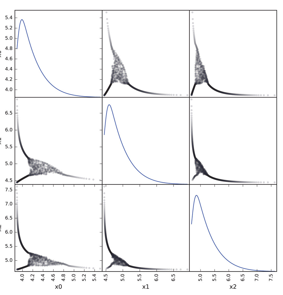
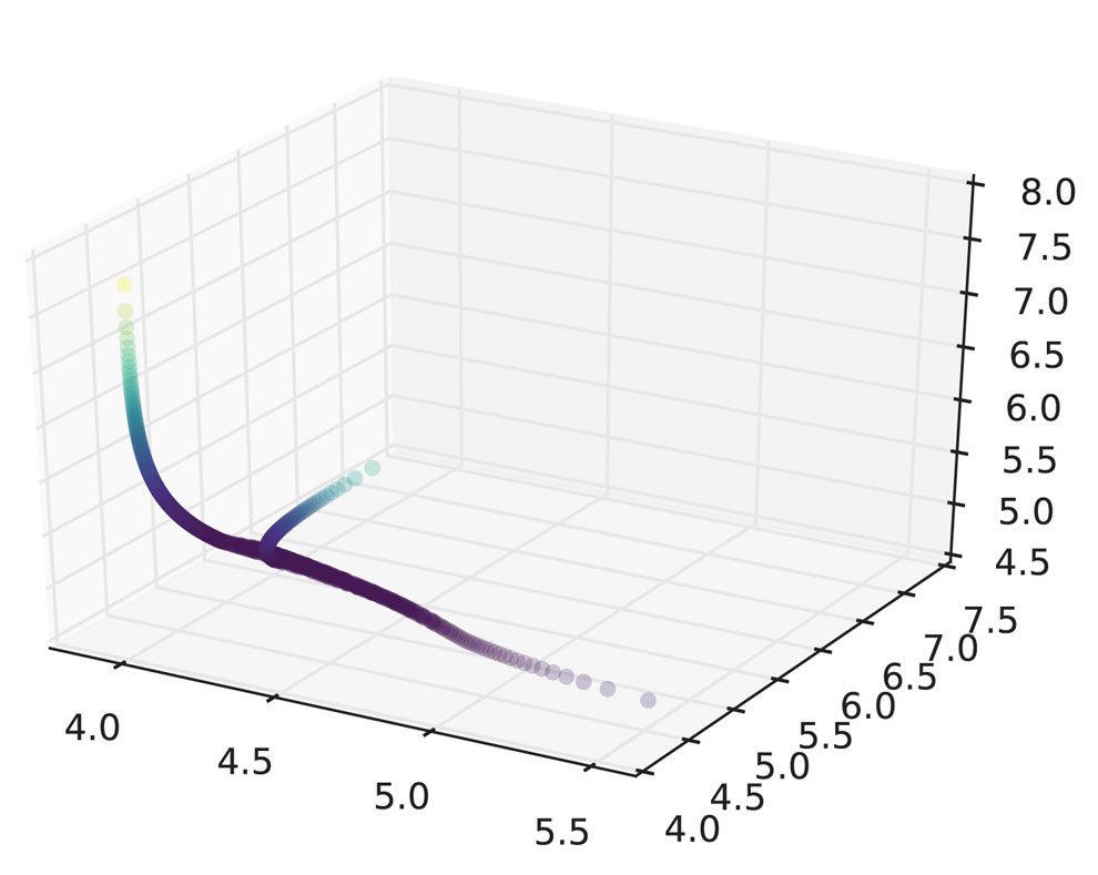
Performing the same calculation with N=1000 samples from the largest 1 percent of each marginal produces an estimated worst VaR of 360.5. Figure 1 shows plots of the marginals with the worst VaR dependence structure, highlighting the same concepts shown in Table 1. The diagonal plots show histograms of each marginal. Working with even larger values of N does not change the result significantly. Figure 2 reveals the strange dependence between the marginals by plotting in three dimensions.
Just as for the case d=2, there are several important points to note about the Re-Arrangement Algorithm output and the failure of subadditivity it induces.
- The algorithm works for any non-trivial marginal distributions — it is universal.
- The output is tailored to a specific value of a and does not work for other values of a. It will actually produce relatively thinner tails for higher values of a than the comonotonic copula. In Table 1 the comonotonic sum is greater than the maximum VaR sum for the top 40 percent of observations, above 366.4.
- The implied dependence structure only specifies how the larger values of each marginal are related; for values below VaRα, any dependence structure can be used.
- The dependence structure does not have right tail dependence.
The Re-Arrangement Algorithm is easy to program and can be applied in cases with hundreds of thousands of simulations and hundreds or more marginals. It gives a definitive answer to the question “Just how bad could things get?” and, perhaps, provides a better base against which to measure the diversification effect than either independence or the comonotonic copula. It is a valuable additional feature for any risk aggregation software. While the multivariate structure it reveals is odd and specific to α, it can’t be dismissed as wholly improbable. It pinpoints a worst case driven by a combination of moderately severe, but not absolutely extreme, tail event outcomes. Anyone who remembers watching their investment portfolio during the financial crisis has seen that behavior before!
Next issue’s column will discuss the two remaining ways subadditivity fails: extreme skewness and the bizarre world of extremely thick tails.
Bibliography
Embrechts, Paul, Giovanni Puccetti and Ludger Ruschendorf. 2013. “Model uncertainty and VaR aggregation.” Journal of Banking and Finance 37 (8):2750–64. https://doi.org/10.1016/j.jbankfin.2013.03.014.
Puccetti, Giovanni, and Ludger Ruschendorf. 2012. “Computation of sharp bounds on the distribution of a function of dependent risks.” Journal of Computational and Applied Mathematics 236 (7). Elsevier B.V.:1833–40. https://doi.org/10.1016/j.cam.2011.10.015.
AR Explorations Editor Stephen Mildenhall, FCAS, CERA, Ph.D., is an assistant professor of risk management and insurance and director of insurance data analytics at the School of Risk Management in the Tobin College of Business at St. John’s University.